Showing posts with label Algorithms. Show all posts

2012-08-06

Merge Right

The so-called master-transaction update is one of the, if not the defining algorithms of the discipline formerly known as "data processing". Given two sorted files of records with increasing keys, the process applies each record in the transaction file to each record of the the master file and outputs the result, if any, to the updated master file in one pass over each input. The same algorithm can compute the union, intersection or difference of sorted sequences. For instance, the union of two sets represented as sorted lists of unique elements is:

let union       =
  let rec go l r = match l, r with
  | [], xs | xs, []  -> xs
  | x :: xs, y :: ys ->
    match compare x y with
    | -1 -> x :: go       xs (y :: ys)
    |  0 -> x :: go       xs       ys
    |  1 -> y :: go (x :: xs)      ys
    |  _ -> assert false
  in go

Intersection is:

let inter       =
  let rec go l r = match l, r with
  | [], _  | _, []   -> []
  | x :: xs, y :: ys ->
    match compare x y with
    | -1 ->      go       xs (y :: ys)
    |  0 -> x :: go       xs       ys
    |  1 ->      go (x :: xs)      ys
    |  _ -> assert false
  in go

while difference is:

let diff       =
  let rec go l r = match l, r with
  | [], _  | _, []   -> l
  | x :: xs, y :: ys ->
    match compare x y with
    | -1 -> x :: go       xs (y :: ys)
    |  0 ->      go       xs       ys
    |  1 ->      go (x :: xs)      ys
    |  _ -> assert false
  in go

And so on. The three functions use the same underlying merge schemata; what varies is the operation to perform in each of the five possible cases:

  1. The left sequence is nil
  2. The right sequence is nil
  3. The next element in the left sequence is less than the next element in the right sequence
  4. The next element in the left sequence is equal to the next element in the right sequence
  5. The next element in the left sequence is greater than the next element in the right sequence

The question is, then, how many set operations can the merge algorithm implement? These five cases partition both input sequences in disjoint sets such that the output sequence is the natural merge of zero or more of them. For example, processing the sets { 1, 3, 4, 6, 7, 8 } ⋈ { 2, 3, 5, 6, 8, 9 } results in the following steps:

LNRNLTEQGTArguments
1 { 1, 3, 4, 6, 7, 8 } ⋈ { 2, 3, 5, 6, 8, 9, 10 }
2{ 3, 4, 6, 7, 8 } ⋈ { 2, 3, 5, 6, 8, 9, 10 }
3 { 3, 4, 6, 7, 8 } ⋈ { 3, 5, 6, 8, 9, 10 }
4 { 4, 6, 7, 8 } ⋈ { 5, 6, 8, 9, 10 }
5{ 6, 7, 8 } ⋈ { 5, 6, 8, 9, 10 }
6 { 6, 7, 8 } ⋈ { 6, 8, 9, 10 }
7 { 7, 8 } ⋈ { 8, 9, 10 }
8 { 8 } ⋈ { 9, 10 }
9,10∅ ⋈ { 9, 10 }

Abstracting away the operations to perform in each of these five cases we have the following schema:

let merge ln rn lt eq gt : 'a list -> 'a list -> 'a list =
  let rec go l r = match l, r with
  | [], ys -> ln ys
  | xs, [] -> rn xs
  | x :: xs, y :: ys ->
    match compare x y with
    | -1 -> lt x (go       xs (y :: ys))
    |  0 -> eq x (go       xs       ys )
    |  1 -> gt y (go (x :: xs)      ys )
    |  _ -> assert false
  in go

Both ln and rn must decide what to do with the remaining list and so have type α list → α list, while lt, eq and gt must decide what to do with the element in consideration and so have type αα list → α list; thus the type of merge is (α list → α list) → (α list → α list) → (αα list → α list) → (αα list → α list) → (αα list → α list) → α list → α list → α list. The operations on the remainder either pass it unchanged or return nil, while the operations on the next element either add it to the output sequence or not:

let self   xs =      xs
and null   _  =      []
and cons x xs = x :: xs
and tail _ xs =      xs

(some of these have well-known names in functional programming, but here I choose to use these neat, four-letter ones.) With the proviso that the output sequence must be increasing these four functions exhaust the possibilities by parametricity; otherwise, duplications and rearrangements would satisfy the parametric signature. Now union, intersection and difference are simply:

let union l r = merge self self  cons cons cons l r
and inter l r = merge null null  tail cons tail l r
and diff  l r = merge null self  cons tail tail l r

It is obvious that the question I posed above is answered as 25 = 32 possible set operations obtainable by varying each of the five operations. The next question is, then, what are these 32 operations? Let me characterize each of the five sets ln, rn, lt, eq and gt. The easiest one is eq, as it obviously is the intersection of both sets:

eq(A, B) = A ∩ B

By substitution in merge it is possible to show that ln(A, B) = rn(B, A) and vice versa; hence just one set expression suffices. The merge ends with rn for every element in A that is greater than every element in B, as the latter were included in the comparison sets; and conversely for ln. Hence:

ln(A, B) = B / A ≡ ⟨S y : B : ⟨∀ x : A : y > x⟩⟩
rn(A, B) = A / B ≡ ⟨S x : A : ⟨∀ y : B : x > y⟩⟩

(read A / B as "A over B"). All three sets are pairwise disjoint, since A / B ⊆ A and A / B ∩ B = ∅, and conversely, by construction.

The two remaining sets are also symmetric in the sense that lt(A, B) = gt(B, A) but are more difficult to characterize. My first attempt was to think of each element in A as being processed in turn and put into lt(A, B) just when strictly less than all the elements in B against which it could be matched, namely lt(A, B) = ⟨S x : A : x < ⟨min y : B : x ≤ y⟩⟩. The condition can be simplified with a bit of equational reasoning:

   x∈A ∧ x < ⟨min y : B : x ≤ y⟩
≡ { GLB }
   x∈A ∧ ⟨∀ y : y∈B ∧ x ≤ y : x < y⟩⟩
≡ { Trading }
   x∈A ∧ ⟨∀ y : y∈B : x > y ∨ x < y⟩⟩
≡ { Trichotomy }
   x∈A ∧ ⟨∀ y : y∈B : x ≠ y⟩⟩
≡
   x∈A ∧ x∉B

In other words, A − B. The problem is that, since the quantification over an empty set is trivially true, this set is too big as it includes the respective remainder; that is to say A / B ⊆ A − B as I showed above. To preserve disjointness I define:

lt(A, B) = A − B − A / B
gt(A, B) = B − A − B / A

In a Venn diagram, these five sets are:

Venn diagram of the five component sets

So by including or excluding one of the five components depending on the function passed to each of the five operations, the 32 set operations achievable by merge are:

Venn diagrams for all 32 set operations

Or in tabular form:

NlnrnlteqgtFunction
0selfselfconsconsconsA∪B
1selfselfconsconstailA B/A
2selfselfconstailconsA∆B
3selfselfconstailtailA−BB/A
4selfselftailconsconsB A/B
5selfselftailconstailA∩BB/AA/B
6selfselftailtailconsB−AA/B
7selfselftailtailtail B/AA/B
8selfnullconsconsconsA∪BA/B
9selfnullconsconstailA B/AA/B
10selfnullconstailconsA∆BA/B
11selfnullconstailtailA−BB/AA/B
12selfnulltailconsconsB
13selfnulltailconstailA∩BB/A
14selfnulltailtailconsB−A
15selfnulltailtailtail B/A
16nullselfconsconsconsA∪BB/A
17nullselfconsconstailA
18nullselfconstailconsA∆BB/A
19nullselfconstailtailA−B
20nullselftailconsconsB B/AA/B
21nullselftailconstailA∩BA/B
22nullselftailtailconsB−AB/AA/B
23nullselftailtailtail A/B
24nullnullconsconsconsA∪BB/AA/B
25nullnullconsconstailA A/B
26nullnullconstailconsA∆BB/AA/B
27nullnullconstailtailA−BA/B
28nullnulltailconsconsB B/A
29nullnulltailconstailA∩B
30nullnulltailtailconsB−AB/A
31nullnulltailtailtail

Arguably, besides the traditional five set operations A ∪ B, A ∩ B, A − B, B − A and A ∆ B, only the remainders A / B, B / A and perhaps A / B ∪ B / A = A ⊔ B, the join of A and B (not to be confused with the relational operation), are independently useful. These three are obscure, and as far as I know have no name, although I'd love to hear if there is literature about them. This might mean that this exhaustive catalog of set merges is rather pointless, but at least now I know for sure.

2012-07-12

A minor branch off Braun Trees

Revisiting the post on Braun Trees I noticed that, while pedagogical, the implementation of the root replacement operation rep can be streamlined a bit. By inlining the mutually recursive siftdown, specializing on the matches and adding guards, the result is as follows:

let rec rep compare e = function
| N (_, (N (el, _, _) as l), E)
  when compare el e  < 0 ->
  N (el, rep compare e l, E)
| N (_, (N (el, _, _) as l), (N (er, _, _) as r))
  when compare el e  < 0
    || compare er e  < 0 ->
    if compare el er < 0
      then N (el, rep compare e l, r)
      else N (er, l, rep compare e r)
| N (_, l, r) -> N (e, l, r)
| E           -> failwith "empty heap"

The guards are the strongest possible in order to minimize the needs to descend to the children. The conditional under the second case could be in turn lifted to a guard, since (el < eer < e) ∧ el < erel < eel < er, and similarly for the else case, but the loss of simplicity is quite substantial in my opinion.

2012-06-29

2D Interpolation, Part 5: Final Optimizations

The code has now the proper shape to carry out optimizations to their logical consequences, to the point that I question the wisdom in some of the previous transformations. It is true that in compiler construction some passes introduce constructs only for latter passes to eliminate them, in the hope of an overall simplification. In this case the starting point will be the elimination of the pixel-for-pixel dispatch to the required interpolator, by hoisting the switch out of the inner loop to a top-level procedure. I keep the last version of the interpolator as interp1 applying the same trick I used before to compare pixels:

void interp0() {
  switch (method) {
  case NEAREST:  interpN(); break;
  case BILINEAR: interpL(); break;
  case BICUBIC:  interpC(); break;
  }
}

The initial version of these interpolators are three identical copies of the previous interp0, appropriately renamed. For the sake of brevity I will omit these copies, showing instead the final, simplified form of each one. In the case of interpN(), I first eliminate the switch. Then I eliminate all references to the repeated border (variables having 0 or 3 as indices). Since there is no need to repeat elements, I now can access the source array directly. This in turn allows me to simplify all index computations, adjusting the condition on the last column as required. In fact, there is no need to keep count of the rows as yi already does that, so the end condition on the outer loop gets radically simpler. A further optimization I can afford is to eliminate the need for floating point constants yf, xf by inlining the integer calculation directly into the conditional:

void interpN() {
  int yr = 0;
  int yi = 1;
  int offset = 0;
  for (int i = 0; i < height; i++) {
    int c11 = srcpix[(yi-1)*ncols+0], c12 = srcpix[(yi-1)*ncols+1];
    int c21 = srcpix[ yi   *ncols+0], c22 = srcpix[ yi   *ncols+1];
    int xr = 0;
    int xi = 1;
    for (int j = 0; j < width; j++) {
      final int c = 2*yr < height ? 2*xr < width ? c11 : c12 : 2*xr < width ? c21 : c22;
      pixels[offset++] = c;
      xr += ncols - 1;
      if (xr >= width) {
        xr -= width;
        xi += 1;
        if (xi < ncols) {
          c11 = c12; c12 = srcpix[(yi-1)*ncols+xi];
          c21 = c22; c22 = srcpix[ yi   *ncols+xi];
        }
      }
    }
    yr += nrows - 1;
    if (yr >= height) {
      yr -= height;
      yi += 1;
    }
  }
}

The simplification on the linear interpolator interpL() proceeds exactly as before. The access pattern is identical, since the stencil is 2×2, so the end result is the same except for the pixel calculation:

void interpL() {
  int yr = 0;
  int yi = 1;
  int offset = 0;
  for (int i = 0; i < height; i++) {
    final float yf = (float) yr / (float) height;
    int c11 = srcpix[(yi-1)*ncols+0], c12 = srcpix[(yi-1)*ncols+1];
    int c21 = srcpix[ yi   *ncols+0], c22 = srcpix[ yi   *ncols+1];
    int xr = 0;
    int xi = 1;
    for (int j = 0; j < width; j++) {
      final float xf = (float) xr / (float) width;
      final int c = bilinear(xf, yf, c11, c12, c21, c22);
      pixels[offset++] = c;
      xr += ncols - 1;
      if (xr >= width) {
        xr -= width;
        xi += 1;
        if (xi < ncols) {
          c11 = c12; c12 = srcpix[(yi-1)*ncols+xi];
          c21 = c22; c22 = srcpix[ yi   *ncols+xi];
        }
      }
    }
    yr += nrows - 1;
    if (yr >= height) {
      yr -= height;
      yi += 1;
    }
  }
}

This leaves me with the bicubic interpolator interpC(). On the one hand there is no need nor possibility to change anything besides eliminating the switch, as all previous transformations were based on the use of a 4×4 stencil with repetitions. On the other, I always question myself whether I can do better. I reason as follows: the stencil ranges over the image from pixel (-1, -1) to pixel (width−3, height−3); in case of under- or overflow the missing pixels are repeated. This means that using min and max as needed can fetch the repetitions for free! In general, the index will be min(max(yi-d, 0),nrows-1), but depending on the value of d and knowing the range of yi some simplifications are possible. The same is true for the repetition of the last column. In the inner loop I use the same trick I did with the arrayCopy(), that is, move the old pixels and fetch the new only if in range:

void interpC() {
  int yr = 0;
  int yi = 2;
  int offset = 0;
  for (int i = 0; i < height; i++) {
    final float yf = (float) yr / (float) height;
    int c00 = srcpix[max(yi-3,     0)*ncols+0];
    int c01 = srcpix[max(yi-3,     0)*ncols+0];
    int c02 = srcpix[max(yi-3,     0)*ncols+1];
    int c03 = srcpix[max(yi-3,     0)*ncols+2];
    int c10 = srcpix[   (yi-2       )*ncols+0];
    int c11 = srcpix[   (yi-2       )*ncols+0];
    int c12 = srcpix[   (yi-2       )*ncols+1];
    int c13 = srcpix[   (yi-2       )*ncols+2];
    int c20 = srcpix[   (yi-1       )*ncols+0];
    int c21 = srcpix[   (yi-1       )*ncols+0];
    int c22 = srcpix[   (yi-1       )*ncols+1];
    int c23 = srcpix[   (yi-1       )*ncols+2];
    int c30 = srcpix[min(yi  ,nrows-1)*ncols+0];
    int c31 = srcpix[min(yi  ,nrows-1)*ncols+0];
    int c32 = srcpix[min(yi  ,nrows-1)*ncols+1];
    int c33 = srcpix[min(yi  ,nrows-1)*ncols+2];
    int xr = 0;
    int xi = 2;
    for (int j = 0; j < width; j++) {
      final float xf = (float) xr / (float) width;
      final int c = bicubic(xf, yf,
            c00, c01, c02, c03, c10, c11, c12, c13,
            c20, c21, c22, c23, c30, c31, c32, c33);
      pixels[offset++] = c;
      xr += ncols - 1;
      if (xr >= width) {
        xr -= width;
        xi += 1;
        c00 = c01; c01 = c02; c02 = c03;
        c10 = c11; c11 = c12; c12 = c13;
        c20 = c21; c21 = c22; c22 = c23;
        c30 = c31; c31 = c32; c32 = c33;
        if (xi < ncols) {
          c03 = srcpix[max(yi-3,      0)*ncols+xi];
          c13 = srcpix[   (yi-2        )*ncols+xi];
          c23 = srcpix[   (yi-1        )*ncols+xi];
          c33 = srcpix[min(yi  ,nrows-1)*ncols+xi];
        }
      }
    }
    yr += nrows - 1;
    if (yr >= height) {
      yr -= height;
      yi += 1;
    }
  }
}

Note that the stencil is loaded at the top of the inner loop with full knowledge of the values that yi and xi can take. Note also that eliminating the conditions implicit in the min and max calculations would require inverting the loops so that the control variables are yi and xi. This is possible but would require modular arithmetic on the destination indices; I would have to start the overall process from scratch.

In the mean time, I suspect that the introduction of row buffers was a red herring (although I swear an innocent, unwitting one). I didn't think of using min and max until the code was focused enough for me to see it from another side. What with insight it appears perfectly obvious can be and often is obscured by unrelated considerations. Selecting the "best" strategy at each step requires knowing the full path to the goal, but when faced with limited information the best we can hope for is that our heuristics don't mislead us too far away. In any case backtracking is inevitable for those of us lacking the gift of foreknowledge, and I think much more honest (if boring) to fully disclose my veering into blind alleys.

The take-away lesson of this (admittedly repetitious, if not downright tedious) exercise is to show how to manually apply some of the strategies that modern parallelizing compilers use automatically to vectorize and optimize straight-loop code, including the use of comparisons with unoptimized versions to assess and ensure the correctness of the transformations. When faced with optimized code I am often left wondering what process the author followed to arrive at that result; my own process is rather pedestrian and methodical and without any magic tricks other than a basic knowledge of high-school arithmetic.

2012-06-28

2D Interpolation, Part 4: ARGB Interpolation

After linearizing all array accesses, interpolating ARGB values is easy from the algorithmic side of things; so easy things first. I'll handle the pixel interpolation proper by abstracting them away in their own little functions. Processing an ARGB source array is just a matter of changing the variable declarations:

final int[] srcpix = {
0xff0051ff, 0xff00fffb, 0xff9cff00, 0xff0051ff,
0xffff0000, 0xff00ff08, 0xffffdb00, 0xff00fffb,
0xff9cff00, 0xff00fffb, 0xff0051ff, 0xffffdb00,
0xffffdb00, 0xff9cff00, 0xff00fffb, 0xff00ff08,
};
final int nrows = 4;
final int ncols = 4;

void interp0() {
  final int[] p = new int[4*ncols+8];
  p[1*ncols+2] = srcpix[0*ncols]; arrayCopy(srcpix, 0*ncols, p, 1*ncols+3, ncols); p[2*ncols+3] = srcpix[1*ncols-1];
  p[2*ncols+4] = srcpix[1*ncols]; arrayCopy(srcpix, 1*ncols, p, 2*ncols+5, ncols); p[3*ncols+5] = srcpix[2*ncols-1];
  p[3*ncols+6] = srcpix[2*ncols]; arrayCopy(srcpix, 2*ncols, p, 3*ncols+7, ncols); p[4*ncols+7] = srcpix[3*ncols-1];
  arrayCopy(p, 1*ncols+2, p, 0, ncols+2);
  int yr = 0;
  int yi = 2;
  int offset = 0;
  for (int i = 0; i < height; i++) {
    final float yf = (float) yr / (float) height;
    int c00 = p[0*ncols+0], c01 = p[0*ncols+1], c02 = p[0*ncols+2], c03 = p[0*ncols+3];
    int c10 = p[1*ncols+2], c11 = p[1*ncols+3], c12 = p[1*ncols+4], c13 = p[1*ncols+5];
    int c20 = p[2*ncols+4], c21 = p[2*ncols+5], c22 = p[2*ncols+6], c23 = p[2*ncols+7];
    int c30 = p[3*ncols+6], c31 = p[3*ncols+7], c32 = p[3*ncols+8], c33 = p[3*ncols+9];
    int xr = 0;
    int xi = 3;
    for (int j = 0; j < width; j++) {
      final float xf = (float) xr / (float) width;
      int c = 0;
      switch (method) {
      case NEAREST:
        c = yf < 0.5 ? xf < 0.5 ? c11 : c12 : xf < 0.5 ? c21 : c22;
        break;
      case BILINEAR:
        c = bilinear(xf, yf, c11, c12, c21, c22);
        break;
      case BICUBIC:
        c = bicubic(xf, yf,
                    c00, c01, c02, c03, c10, c11, c12, c13,
                    c20, c21, c22, c23, c30, c31, c32, c33);
        break;
      }
      pixels[offset++] = c;
      xr += ncols - 1;
      if (xr >= width) {
        xr -= width;
        xi += 1;
        if (xi < ncols+2) {
          c00 = c01; c01 = c02; c02 = c03; c03 = p[0*ncols+xi+0];
          c10 = c11; c11 = c12; c12 = c13; c13 = p[1*ncols+xi+2];
          c20 = c21; c21 = c22; c22 = c23; c23 = p[2*ncols+xi+4];
          c30 = c31; c31 = c32; c32 = c33; c33 = p[3*ncols+xi+6];
        }
      }
    }
    yr += nrows - 1;
    if (yr >= height) {
      yr -= height;
      yi += 1;
      if (yi <= nrows) {
        arrayCopy(p, (ncols+2), p, 0, 3*(ncols+2));
        if (yi < nrows) {
          p[3*ncols+6] = srcpix[yi*ncols];
          arrayCopy(srcpix, yi*ncols, p, 3*ncols+7, ncols);
          p[4*ncols+7] = srcpix[(yi+1)*ncols-1];
        }
      }
    }
  }
}

The pixel array is the result of obtaining the hue() for each value in the original float array data. As you can see, I simplified the inner switch by extracting the interpolation schemes off to named routines. These routines will have to unpack the four components in each pixel, interpolate each component and pack back the result pixel. The bilinear interpolator is straightforward:

static int bilinear(final float t, final float u,
                    final int c00, final int c01,
                    final int c10, final int c11) {
  final int a00=(c00>>24)&0xff, r00=(c00>>16)&0xff, g00=(c00>>8)&0xff, b00=c00&0xff;
  final int a01=(c01>>24)&0xff, r01=(c01>>16)&0xff, g01=(c01>>8)&0xff, b01=c01&0xff;
  final int a10=(c10>>24)&0xff, r10=(c10>>16)&0xff, g10=(c10>>8)&0xff, b10=c10&0xff;
  final int a11=(c11>>24)&0xff, r11=(c11>>16)&0xff, g11=(c11>>8)&0xff, b11=c11&0xff;
  final float a = linear(u, linear(t, a00, a01), linear(t, a10, a11));
  final float r = linear(u, linear(t, r00, r01), linear(t, r10, r11));
  final float g = linear(u, linear(t, g00, g01), linear(t, g10, g11));
  final float b = linear(u, linear(t, b00, b01), linear(t, b10, b11));
  return (int) a << 24 | (int) r << 16 | (int) g << 8 | (int) b;

Note that the pixels are unpacked in "row" (ARGB) order but interpolated in "column" order; these transpositions are typical of vectorized and GPU code. The result is very different to the previous version of the linear interpolator, since I'm interpolating vectors here, not scalars mapped to a color ramp:

bilinear interpolation

You can see very noticeable Mach banding in the form of color ridges and creases. hue() mitigated this effect by smootherstep'ping the parameter, and I can do the same here, by converting a float channel into a saturated (that is, range limited) int channel:

static int bsat(float x) {
  if (x < 0)
    return 0;
  else if (x > 255)
    return 255;
  x /= 255f;
  return (int) ((10 - (15 - 6 * x) * x) * x * x * x * 255);
}

Changing the last line in bilinear() to:

  return bsat(a) << 24 | bsat(r) << 16 | bsat(g) << 8 | bsat(b);

results in an image with the high-frequency components smoothed out or filtered:

bilinear interpolation with smoothing

Much nicer. In fact I now understand why there are so many interpolation options to resize an image in Adobe Photoshop®. In the case of the bicubic interpolation I quickly learned that some sort of clipping and/or rescaling is vital, since the "tension" given by the derivatives can make the interpolated values overshoot:

bicubic interpolation with channel overflow errors

This is easily seen by masking out every channel but one:

bicubic interpolation with channel overflow errors, red channel

In fact, a little experimentation shows that interpolated values can go as low as -72 or as high as 327! The worst outliers are, of course, the result of interpolating high-frequency matrices of the form [[0 1 1 0] [1 0 0 1] [1 0 0 1] [0 1 1 0]]. Local rescaling is not a good choice, in my opinion, since it would wash out all channels equally; in particular, it would make images more transparent than they really are. The obvious choice is clipping, although doing that without filtering introduces artifacts:

bicubic interpolation with clipping

Using the bsat() above produces the best results:

bicubic interpolation with clipping and smoothing

The final code for the ARGB bicubic interpolator is:

static int bicubic(final float t, final float u,
                   final int c00, final int c01, final int c02, final int c03,
                   final int c10, final int c11, final int c12, final int c13,
                   final int c20, final int c21, final int c22, final int c23,
                   final int c30, final int c31, final int c32, final int c33) {
  final int a00=(c00>>24)&0xff, r00=(c00>>16)&0xff, g00=(c00>>8)&0xff, b00=c00&0xff;
  final int a01=(c01>>24)&0xff, r01=(c01>>16)&0xff, g01=(c01>>8)&0xff, b01=c01&0xff;
  final int a02=(c02>>24)&0xff, r02=(c02>>16)&0xff, g02=(c02>>8)&0xff, b02=c02&0xff;
  final int a03=(c03>>24)&0xff, r03=(c03>>16)&0xff, g03=(c03>>8)&0xff, b03=c03&0xff;
  final int a10=(c10>>24)&0xff, r10=(c10>>16)&0xff, g10=(c10>>8)&0xff, b10=c10&0xff;
  final int a11=(c11>>24)&0xff, r11=(c11>>16)&0xff, g11=(c11>>8)&0xff, b11=c11&0xff;
  final int a12=(c12>>24)&0xff, r12=(c12>>16)&0xff, g12=(c12>>8)&0xff, b12=c12&0xff;
  final int a13=(c13>>24)&0xff, r13=(c13>>16)&0xff, g13=(c13>>8)&0xff, b13=c13&0xff;
  final int a20=(c20>>24)&0xff, r20=(c20>>16)&0xff, g20=(c20>>8)&0xff, b20=c20&0xff;
  final int a21=(c21>>24)&0xff, r21=(c21>>16)&0xff, g21=(c21>>8)&0xff, b21=c21&0xff;
  final int a22=(c22>>24)&0xff, r22=(c22>>16)&0xff, g22=(c22>>8)&0xff, b22=c22&0xff;
  final int a23=(c23>>24)&0xff, r23=(c23>>16)&0xff, g23=(c23>>8)&0xff, b23=c23&0xff;
  final int a30=(c30>>24)&0xff, r30=(c30>>16)&0xff, g30=(c30>>8)&0xff, b30=c30&0xff;
  final int a31=(c31>>24)&0xff, r31=(c31>>16)&0xff, g31=(c31>>8)&0xff, b31=c31&0xff;
  final int a32=(c32>>24)&0xff, r32=(c32>>16)&0xff, g32=(c32>>8)&0xff, b32=c32&0xff;
  final int a33=(c33>>24)&0xff, r33=(c33>>16)&0xff, g33=(c33>>8)&0xff, b33=c33&0xff;
  final float a = cubic(u, cubic(t, a00, a01, a02, a03), cubic(t, a10, a11, a12, a13),
                           cubic(t, a20, a21, a22, a23), cubic(t, a30, a31, a32, a33));
  final float r = cubic(u, cubic(t, r00, r01, r02, r03), cubic(t, r10, r11, r12, r13),
                           cubic(t, r20, r21, r22, r23), cubic(t, r30, r31, r32, r33));
  final float g = cubic(u, cubic(t, g00, g01, g02, g03), cubic(t, g10, g11, g12, g13),
                           cubic(t, g20, g21, g22, g23), cubic(t, g30, g31, g32, g33));
  final float b = cubic(u, cubic(t, b00, b01, b02, b03), cubic(t, b10, b11, b12, b13),
                           cubic(t, b20, b21, b22, b23), cubic(t, b30, b31, b32, b33));
  return bsat(a) << 24 | bsat(r) << 16 | bsat(g) << 8 | bsat(b);
}

Quite a mouthful, but I arrived at it by methodic and meticulous columnar editing. Now everything is ready to tackle the problem of hoisting the conditional in the inner loop and deriving three different, fully streamlined interpolators. Until next time.

2012-06-27

2D Interpolation, Part 3: Linear Array Accesses

Last time I've hoisted all accesses to the source array. This opens the door to being able to process linear arrays representing a matrix in row-major order by stenciling. Not only that, but I was able to completely eliminate the need to have a bordered array on input by explicitly replicating elements as needed. The first step is to use a row buffer into which to copy the elements to be processed. Instead of stenciling by indexing into the source array, I'll index into this row buffer. The code is identical to the one presented last time, except for the initialization, done by copying, and the indexing. Instead of four arrays p0, p1, p2 and p3 I use just one containing four rows back to front; this requires computing the indices by hand. To bring in the next row to interpolate, a pair of arrayCopys make room in the row buffer and assign the new row in the opened space. Now both yi and xi cease to represent the index of the stencil over the source array, and I'm free to simplify the index arithmetic by offsetting their starting values:

void interp0() {
  final float[] p = new float[4 * nx];
  for (int i = 0; i < 4; i++)
    arrayCopy(data[i], 0, p, i*nx, nx);
  int yr = 0;
  int yi = 3;
  int offset = 0;
  for (int i = 0; i < height; i++) {
    final float yf = (float) yr / (float) height;
    float c00 = p[0*nx+0], c01 = p[0*nx+1], c02 = p[0*nx+2], c03 = p[0*nx+3];
    float c10 = p[1*nx+0], c11 = p[1*nx+1], c12 = p[1*nx+2], c13 = p[1*nx+3];
    float c20 = p[2*nx+0], c21 = p[2*nx+1], c22 = p[2*nx+2], c23 = p[2*nx+3];
    float c30 = p[3*nx+0], c31 = p[3*nx+1], c32 = p[3*nx+2], c33 = p[3*nx+3];
    int xr = 0;
    int xi = 3;
    for (int j = 0; j < width; j++) {
      final float xf = (float) xr / (float) width;
      float c = 0;
      switch (method) {
      case NEAREST:
        c = yf < 0.5 ? xf < 0.5 ? c11 : c12 : xf < 0.5 ? c21 : c22;
        break;
      case BILINEAR:
        c = linear(yf,
            linear(xf, c11, c12),
            linear(xf, c21, c22) );
        break;
      case BICUBIC:
        c = cubic(yf,
            cubic(xf, c00, c01, c02, c03),
            cubic(xf, c10, c11, c12, c13),
            cubic(xf, c20, c21, c22, c23),
            cubic(xf, c30, c31, c32, c33) );
        break;
      }
      pixels[offset++] = hue(c);
      xr += nx - 3;
      if (xr >= width) {
        xr -= width;
        xi += 1;
        if (xi < nx) {
          c00 = c01; c01 = c02; c02 = c03; c03 = p[0*nx+xi];
          c10 = c11; c11 = c12; c12 = c13; c13 = p[1*nx+xi];
          c20 = c21; c21 = c22; c22 = c23; c23 = p[2*nx+xi];
          c30 = c31; c31 = c32; c32 = c33; c33 = p[3*nx+xi];
        }
      }
    }
    yr += ny - 3;
    if (yr >= height) {
      yr -= height;
      yi += 1;
      if (yi < ny) {
        arrayCopy(p, nx, p, 0, 3*nx);
        arrayCopy(data[yi], 0, p, 3*nx, nx);
      }
    }
  }
}

Processing a matrix as a linear array in row-major order is a matter of adjusting the sources to the arrayCopys. I've renamed the source array as srcpix and its dimensions as nrows and ncols so that later I can modify the code to avoid the need for an explicit border without breaking the existing interp1():

final float[] srcpix = {
  0.60, 0.60, 0.48, 0.24, 0.60, 0.60,
  0.60, 0.60, 0.48, 0.24, 0.60, 0.60,
  0.00, 0.00, 0.36, 0.12, 0.48, 0.48,
  0.24, 0.24, 0.48, 0.60, 0.12, 0.12,
  0.12, 0.12, 0.24, 0.48, 0.36, 0.36,
  0.12, 0.12, 0.24, 0.48, 0.36, 0.36
};
final int nrows = 6;
final int ncols = 6;

void interp0() {
  final float[] p = new float[4 * ncols];
  arrayCopy(srcpix, 0, p, 0, 4 * ncols);
  int yr = 0;
  int yi = 3;
  int offset = 0;
  for (int i = 0; i < height; i++) {
    final float yf = (float) yr / (float) height;
    float c00 = p[0*ncols+0], c01 = p[0*ncols+1], c02 = p[0*ncols+2], c03 = p[0*ncols+3];
    float c10 = p[1*ncols+0], c11 = p[1*ncols+1], c12 = p[1*ncols+2], c13 = p[1*ncols+3];
    float c20 = p[2*ncols+0], c21 = p[2*ncols+1], c22 = p[2*ncols+2], c23 = p[2*ncols+3];
    float c30 = p[3*ncols+0], c31 = p[3*ncols+1], c32 = p[3*ncols+2], c33 = p[3*ncols+3];
    int xr = 0;
    int xi = 3;
    for (int j = 0; j < width; j++) {
      final float xf = (float) xr / (float) width;
      float c = 0;
      switch (method) {
      case NEAREST:
        c = yf < 0.5 ? xf < 0.5 ? c11 : c12 : xf < 0.5 ? c21 : c22;
        break;
      case BILINEAR:
        c = linear(yf,
            linear(xf, c11, c12),
            linear(xf, c21, c22) );
        break;
      case BICUBIC:
        c = cubic(yf,
            cubic(xf, c00, c01, c02, c03),
            cubic(xf, c10, c11, c12, c13),
            cubic(xf, c20, c21, c22, c23),
            cubic(xf, c30, c31, c32, c33) );
        break;
      }
      pixels[offset++] = hue(c);
      xr += ncols - 3;
      if (xr >= width) {
        xr -= width;
        xi += 1;
        if (xi < ncols) {
          c00 = c01; c01 = c02; c02 = c03; c03 = p[0*ncols+xi];
          c10 = c11; c11 = c12; c12 = c13; c13 = p[1*ncols+xi];
          c20 = c21; c21 = c22; c22 = c23; c23 = p[2*ncols+xi];
          c30 = c31; c31 = c32; c32 = c33; c33 = p[3*ncols+xi];
        }
      }
    }
    yr += nrows - 3;
    if (yr >= height) {
      yr -= height;
      yi += 1;
      if (yi < nrows) {
        arrayCopy(p, ncols, p, 0, 3*ncols);
        arrayCopy(srcpix, yi*ncols, p, 3*ncols, ncols);
      }
    }
  }
}

Now in a slow-motion approach towards eliminating the repeated border, I'll first reduce the array dimensions to their true value. In the preceding code I substitute nrows := nrows−2 and ncols := ncols−2, and simplify all indices:

final int nrows = 4;
final int ncols = 4;

void interp0() {
  final float[] p = new float[4*(ncols+2)];
  arrayCopy(srcpix, 0, p, 0, 4*(ncols+2));
  int yr = 0;
  int yi = 3;
  int offset = 0;
  for (int i = 0; i < height; i++) {
    final float yf = (float) yr / (float) height;
    float c00 = p[0*ncols+0], c01 = p[0*ncols+1], c02 = p[0*ncols+2], c03 = p[0*ncols+3];
    float c10 = p[1*ncols+2], c11 = p[1*ncols+3], c12 = p[1*ncols+4], c13 = p[1*ncols+5];
    float c20 = p[2*ncols+4], c21 = p[2*ncols+5], c22 = p[2*ncols+6], c23 = p[2*ncols+7];
    float c30 = p[3*ncols+6], c31 = p[3*ncols+7], c32 = p[3*ncols+8], c33 = p[3*ncols+9];
    int xr = 0;
    int xi = 3;
    for (int j = 0; j < width; j++) {
      final float xf = (float) xr / (float) width;
      float c = 0;
      switch (method) {
      case NEAREST:
        c = yf < 0.5 ? xf < 0.5 ? c11 : c12 : xf < 0.5 ? c21 : c22;
        break;
      case BILINEAR:
        c = linear(yf,
            linear(xf, c11, c12),
            linear(xf, c21, c22) );
        break;
      case BICUBIC:
        c = cubic(yf,
            cubic(xf, c00, c01, c02, c03),
            cubic(xf, c10, c11, c12, c13),
            cubic(xf, c20, c21, c22, c23),
            cubic(xf, c30, c31, c32, c33) );
        break;
      }
      pixels[offset++] = hue(c);
      xr += ncols - 1;
      if (xr >= width) {
        xr -= width;
        xi += 1;
        if (xi < ncols+2) {
          c00 = c01; c01 = c02; c02 = c03; c03 = p[0*ncols+xi+0];
          c10 = c11; c11 = c12; c12 = c13; c13 = p[1*ncols+xi+2];
          c20 = c21; c21 = c22; c22 = c23; c23 = p[2*ncols+xi+4];
          c30 = c31; c31 = c32; c32 = c33; c33 = p[3*ncols+xi+6];
        }
      }
    }
    yr += nrows - 1;
    if (yr >= height) {
      yr -= height;
      yi += 1;
      if (yi < nrows+2) {
        arrayCopy(p, (ncols+2), p, 0, 3*(ncols+2));
        arrayCopy(srcpix, yi*(ncols+2), p, 3*ncols+6, ncols+2);
      }
    }
  }
}

In the second part of the slo-mo maneuver, I'll eliminate the repeated values from the source matrix. Every row repeats the first and last element, and both the first and the last rows are repeated in turn. I achieve this by careful stuffing into the row buffer:

final float[] srcpix = {
0.60, 0.48, 0.24, 0.60,
0.00, 0.36, 0.12, 0.48,
0.24, 0.48, 0.60, 0.12,
0.12, 0.24, 0.48, 0.36,
};
final int nrows = 4;
final int ncols = 4;

void interp0() {
  final float[] p = new float[4*ncols+8];
  p[1*ncols+2] = srcpix[0*ncols]; arrayCopy(srcpix, 0*ncols, p, 1*ncols+3, ncols); p[2*ncols+3] = srcpix[1*ncols-1];
  p[2*ncols+4] = srcpix[1*ncols]; arrayCopy(srcpix, 1*ncols, p, 2*ncols+5, ncols); p[3*ncols+5] = srcpix[2*ncols-1];
  p[3*ncols+6] = srcpix[2*ncols]; arrayCopy(srcpix, 2*ncols, p, 3*ncols+7, ncols); p[4*ncols+7] = srcpix[3*ncols-1];
  arrayCopy(p, 1*ncols+2, p, 0, ncols+2);
  int yr = 0;
  int yi = 2;
  int offset = 0;
  for (int i = 0; i < height; i++) {
    final float yf = (float) yr / (float) height;
    float c00 = p[0*ncols+0], c01 = p[0*ncols+1], c02 = p[0*ncols+2], c03 = p[0*ncols+3];
    float c10 = p[1*ncols+2], c11 = p[1*ncols+3], c12 = p[1*ncols+4], c13 = p[1*ncols+5];
    float c20 = p[2*ncols+4], c21 = p[2*ncols+5], c22 = p[2*ncols+6], c23 = p[2*ncols+7];
    float c30 = p[3*ncols+6], c31 = p[3*ncols+7], c32 = p[3*ncols+8], c33 = p[3*ncols+9];
    int xr = 0;
    int xi = 3;
    for (int j = 0; j < width; j++) {
      final float xf = (float) xr / (float) width;
      float c = 0;
      switch (method) {
      case NEAREST:
        c = yf < 0.5 ? xf < 0.5 ? c11 : c12 : xf < 0.5 ? c21 : c22;
        break;
      case BILINEAR:
        c = linear(yf,
            linear(xf, c11, c12),
            linear(xf, c21, c22) );
        break;
      case BICUBIC:
        c = cubic(yf,
            cubic(xf, c00, c01, c02, c03),
            cubic(xf, c10, c11, c12, c13),
            cubic(xf, c20, c21, c22, c23),
            cubic(xf, c30, c31, c32, c33) );
        break;
      }
      pixels[offset++] = hue(c);
      xr += ncols - 1;
      if (xr >= width) {
        xr -= width;
        xi += 1;
        if (xi < ncols+2) {
          c00 = c01; c01 = c02; c02 = c03; c03 = p[0*ncols+xi+0];
          c10 = c11; c11 = c12; c12 = c13; c13 = p[1*ncols+xi+2];
          c20 = c21; c21 = c22; c22 = c23; c23 = p[2*ncols+xi+4];
          c30 = c31; c31 = c32; c32 = c33; c33 = p[3*ncols+xi+6];
        }
      }
    }
    yr += nrows - 1;
    if (yr >= height) {
      yr -= height;
      yi += 1;
      if (yi <= nrows) {
        arrayCopy(p, (ncols+2), p, 0, 3*(ncols+2));
        if (yi < nrows) {
          p[3*ncols+6] = srcpix[yi*ncols];
          arrayCopy(srcpix, yi*ncols, p, 3*ncols+7, ncols);
          p[4*ncols+7] = srcpix[(yi+1)*ncols-1];
        }
      }
    }
  }
}

Note that during initialization the first row is duplicated by an explicit copy. Note also that the inner loop doesn't change at all. The outer loop does; since the first duplicated row was eliminated, yi initially is 2, not 3; since the last duplicated row was eliminated, there new bounds for yi is nrows, not nrows + 2, and the conditions simplify accordingly. Since the last row is repeated, it must be processed even when yi is exactly nrows. Finally, since the new row must repeat its first and last elements, I must use the same schema as for the initialization. In the case of the repeated last row, the first arrayCopy moves the three last rows to the front; by doing nothing the very last row appears in the last two consecutive strides of the row buffer.

Believe it or not, I consider this code rather compact. Normally, the special case of repeated elements is handled by unrolling the loops and placing a loop header and a loop footer specialized to the appropriate values. By using the row buffer, I can avoid duplicating code, for a cost in O(N) storage. As it is, the only transformation required would be to extract the switch from the inner loop into separate the interpolators and simplify the nearest-neighbor and bilinear cases by eliminating the unneeded elements. Before doing that, it would be best to tackle the problem of processing ARGB sources, by unpacking the channels in the source pixels, interpolating each and repacking them into a destination pixel. That can be done neatly with the row buffers for maximal inner-loop speed. Until the next time!

2012-06-26

2D Interpolation, Part 2: Minimizing Array Accesses

Last time I massaged the interpolator to avoid computing every time the linear transformation from destination space to source space, using only integer variables. With that rewriting, it is time to avoid referencing source values more than is needed. First thing we do, let's name all elements:

void interp0() {
  int offset = 0;
  int yn = 0;
  int yi = 1;
  for (int i = 0; i < height; i++) {
    final float yr = (float) yn / (float) height;
    int xn = 0;
    int xi = 1;
    for (int j = 0; j < width; j++) {
      final float xr = (float) xn / (float) width;
      float c00 = data[yi-1][xi-1], c01 = data[yi-1][xi+0], c02 = data[yi-1][xi+1], c03 = data[yi-1][xi+2];
      float c10 = data[yi+0][xi-1], c11 = data[yi+0][xi+0], c12 = data[yi+0][xi+1], c13 = data[yi+0][xi+2];
      float c20 = data[yi+1][xi-1], c21 = data[yi+1][xi+0], c22 = data[yi+1][xi+1], c23 = data[yi+1][xi+2];
      float c30 = data[yi+2][xi-1], c31 = data[yi+2][xi+0], c32 = data[yi+2][xi+1], c33 = data[yi+2][xi+2];
      float c = 0;
      switch (method) {
      case NEAREST:
        c = yr < 0.5 ? xr < 0.5 ? c11 : c12 : xr < 0.5 ? c21 : c22;
        break;
      case BILINEAR:
        c = linear(yr,
            linear(xr, c11, c12),
            linear(xr, c21, c22) );
        break;
      case BICUBIC:
        c = cubic(yr,
            cubic(xr, c00, c01, c02, c03),
            cubic(xr, c10, c11, c12, c13),
            cubic(xr, c20, c21, c22, c23),
            cubic(xr, c30, c31, c32, c33) );
        break;
      }
      pixels[offset++] = hue(c);
      xn += nx - 3;
      if (xn >= width) {
        xn -= width;
        xi += 1;
      }
    }
    yn += ny - 3;
    if (yn >= height) {
      yn -= height;
      yi += 1;
    }
  }
}

Two things are of note: first, I need all 16 elements for bicubic interpolation, even if nearest-neighbor or bilinear were requested. Second, in the nearest-neighbor case I had to transform an index computation involving a float-to-integer rounding into explicit conditionals. Such is the price of progress.

Since yi, xi don't change at each step, it is possible to just reference new elements when they do, and reuse values in the mean time. First I will reuse the columns. In order to do that I need to hoist the assignments outside the inner loop, in effect converting them to pure initializations, and arrange for the variables to update when xi is incremented:

void interp0() {
  int offset = 0;
  int yn = 0;
  int yi = 1;
  for (int i = 0; i < height; i++) {
    final float yr = (float) yn / (float) height;
    int xn = 0;
    int xi = 1;
    float c00 = data[yi-1][0], c01 = data[yi-1][1], c02 = data[yi-1][2], c03 = data[yi-1][3];
    float c10 = data[yi+0][0], c11 = data[yi+0][1], c12 = data[yi+0][2], c13 = data[yi+0][3];
    float c20 = data[yi+1][0], c21 = data[yi+1][1], c22 = data[yi+1][2], c23 = data[yi+1][3];
    float c30 = data[yi+2][0], c31 = data[yi+2][1], c32 = data[yi+2][2], c33 = data[yi+2][3];
    for (int j = 0; j < width; j++) {
      final float xr = (float) xn / (float) width;
      float c = 0;
      switch (method) {
      case NEAREST:
        c = yr < 0.5 ? xr < 0.5 ? c11 : c12 : xr < 0.5 ? c21 : c22;
        break;
      case BILINEAR:
        c = linear(yr,
            linear(xr, c11, c12),
            linear(xr, c21, c22) );
        break;
      case BICUBIC:
        c = cubic(yr,
            cubic(xr, c00, c01, c02, c03),
            cubic(xr, c10, c11, c12, c13),
            cubic(xr, c20, c21, c22, c23),
            cubic(xr, c30, c31, c32, c33) );
        break;
      }
      pixels[offset++] = hue(c);
      xn += nx - 3;
      if (xn >= width) {
        xn -= width;
        xi += 1;
        if (xi < nx - 2) {
          c00 = c01; c01 = c02; c02 = c03; c03 = data[yi-1][xi+2];
          c10 = c11; c11 = c12; c12 = c13; c13 = data[yi+0][xi+2];
          c20 = c21; c21 = c22; c22 = c23; c23 = data[yi+1][xi+2];
          c30 = c31; c31 = c32; c32 = c33; c33 = data[yi+2][xi+2];
        }
      }
    }
    yn += ny - 3;
    if (yn >= height) {
      yn -= height;
      yi += 1;
    }
  }
}

The initialization inlines the constant value xi = 1 in the second index. The update shifts the values around in classic bucket brigade fashion, and fetches fresh values for the new column to process. Note that there is a subtlety involving the range check, in that the last iteration for j will have xi = nx−2, but at that point it is too early to notice: logically the loop termination test should come before updating xn, xi and the array elements. I opt here to conditionalize the update to keep the for loop structured; feel free to break out of the loop instead.

Now it's time to reuse the rows. This is made simpler by the fact that the source matrix is an array of arrays. First I introduce row variables pointing to each active row, and rename the element accesses accordingly:

void interp0() {
  int offset = 0;
  int yn = 0;
  int yi = 1;
  for (int i = 0; i < height; i++) {
    final float yr = (float) yn / (float) height;
    int xn = 0;
    int xi = 1;
    float[] p0 = data[yi-1], p1 = data[yi+0], p2 = data[yi+1], p3 = data[yi+2];
    float c00 = p0[0], c01 = p0[1], c02 = p0[2], c03 = p0[3];
    float c10 = p1[0], c11 = p1[1], c12 = p1[2], c13 = p1[3];
    float c20 = p2[0], c21 = p2[1], c22 = p2[2], c23 = p2[3];
    float c30 = p3[0], c31 = p3[1], c32 = p3[2], c33 = p3[3];
    for (int j = 0; j < width; j++) {
      final float xr = (float) xn / (float) width;
      float c = 0;
      switch (method) {
      case NEAREST:
        c = yr < 0.5 ? xr < 0.5 ? c11 : c12 : xr < 0.5 ? c21 : c22;
        break;
      case BILINEAR:
        c = linear(yr,
            linear(xr, c11, c12),
            linear(xr, c21, c22) );
        break;
      case BICUBIC:
        c = cubic(yr,
            cubic(xr, c00, c01, c02, c03),
            cubic(xr, c10, c11, c12, c13),
            cubic(xr, c20, c21, c22, c23),
            cubic(xr, c30, c31, c32, c33) );
        break;
      }
      pixels[offset++] = hue(c);
      xn += nx - 3;
      if (xn >= width) {
        xn -= width;
        xi += 1;
        if (xi < nx - 2) {
          c00 = c01; c01 = c02; c02 = c03; c03 = p0[xi+2];
          c10 = c11; c11 = c12; c12 = c13; c13 = p1[xi+2];
          c20 = c21; c21 = c22; c22 = c23; c23 = p2[xi+2];
          c30 = c31; c31 = c32; c32 = c33; c33 = p3[xi+2];
        }
      }
    }
    yn += ny - 3;
    if (yn >= height) {
      yn -= height;
      yi += 1;
    }
  }
}

Next I hoist the row assignments out of the outer loop, as I did before:

void interp0() {
  float[] p0 = data[0], p1 = data[1], p2 = data[2], p3 = data[3];
  int yn = 0;
  int yi = 1;
  int offset = 0;
  for (int i = 0; i < height; i++) {
    final float yr = (float) yn / (float) height;
    float c00 = p0[0], c01 = p0[1], c02 = p0[2], c03 = p0[3];
    float c10 = p1[0], c11 = p1[1], c12 = p1[2], c13 = p1[3];
    float c20 = p2[0], c21 = p2[1], c22 = p2[2], c23 = p2[3];
    float c30 = p3[0], c31 = p3[1], c32 = p3[2], c33 = p3[3];
    int xn = 0;
    int xi = 1;
    for (int j = 0; j < width; j++) {
      final float xr = (float) xn / (float) width;
      float c = 0;
      switch (method) {
      case NEAREST:
        c = yr < 0.5 ? xr < 0.5 ? c11 : c12 : xr < 0.5 ? c21 : c22;
        break;
      case BILINEAR:
        c = linear(yr,
            linear(xr, c11, c12),
            linear(xr, c21, c22) );
        break;
      case BICUBIC:
        c = cubic(yr,
            cubic(xr, c00, c01, c02, c03),
            cubic(xr, c10, c11, c12, c13),
            cubic(xr, c20, c21, c22, c23),
            cubic(xr, c30, c31, c32, c33) );
        break;
      }
      pixels[offset++] = hue(c);
      xn += nx - 3;
      if (xn >= width) {
        xn -= width;
        xi += 1;
        if (xi < nx - 2) {
          c00 = c01; c01 = c02; c02 = c03; c03 = p0[xi+2];
          c10 = c11; c11 = c12; c12 = c13; c13 = p1[xi+2];
          c20 = c21; c21 = c22; c22 = c23; c23 = p2[xi+2];
          c30 = c31; c31 = c32; c32 = c33; c33 = p3[xi+2];
        }
      }
    }
    yn += ny - 3;
    if (yn >= height) {
      yn -= height;
      yi += 1;
      if (yi < ny - 2) {
        p0 = p1; p1 = p2; p2 = p3; p3 = data[yi+2];
      }
    }
  }
}

Here I'm presented with exactly the same situation regarding the last iteration as with the columns, and faced with the same choice. At this point I could call it quits and be satisfied with a reasonable implementation; I'll press further. Next time I'll convert the interpolator to operate on a linear array, opening the door to manipulating graphics directly.

2012-06-25

2D Interpolation, Part 1: The Digital Differential Analyzer

To my Planet OCaml readers, I apologize for veering into Java. I've been playing with Processing of lately, because it's far easier to prototype silly, simple animations (fractals! Fractals everywhere!) in it than by using OCamlSDL, say. Last time I showed a basic 2D interpolator; now it's time to start massaging it into shape. Let's recall the original code:

void interp0() {
  final float dy = (float) (ny - 3) / height;
  final float dx = (float) (nx - 3) / width;
  int offset = 0;
  for (int i = 0; i < height; i++) {
    float yr = 1 + dy * i;
    int yi = (int) yr;
    yr -= yi;
    for (int j = 0; j < width; j++) {
      float xr = 1 + dx * j;
      int xi = (int) xr;
      xr -= xi;
      float c = 0;
      switch (method) {
      case NEAREST:
        c = data[yi + (int) (yr + 0.5)][xi + (int) (xr + 0.5)];
        break;
      case BILINEAR:
        c = linear(yr,
            linear(xr, data[yi+0][xi+0], data[yi+0][xi+1]),
            linear(xr, data[yi+1][xi+0], data[yi+1][xi+1]) );
        break;
      case BICUBIC:
        c = cubic(yr,
            cubic(xr, data[yi-1][xi-1], data[yi-1][xi+0], data[yi-1][xi+1], data[yi-1][xi+2]),
            cubic(xr, data[yi+0][xi-1], data[yi+0][xi+0], data[yi+0][xi+1], data[yi+0][xi+2]),
            cubic(xr, data[yi+1][xi-1], data[yi+1][xi+0], data[yi+1][xi+1], data[yi+1][xi+2]),
            cubic(xr, data[yi+2][xi-1], data[yi+2][xi+0], data[yi+2][xi+1], data[yi+2][xi+2]) );
        break;
      }
      pixels[offset++] = hue(c);
    }
  }
}

The coordinate transformations from destination array to source matrix involve a linear transformation s = s0 + k·(d - d0), where k is a floating-point approximation to a rational number. This can be done using the all-integer Digital Differential Analyzer or DDA. First of all, note that there's no reason for yr, xr to start at 1; only yi, xi need to be offset:

void interp0() {
  final float dy = (float) (ny - 3) / height;
  final float dx = (float) (nx - 3) / width;
  int offset = 0;
  for (int i = 0; i < height; i++) {
    float yr = dy * i;
    int yi = (int) yr;
    yr -= yi;
    yi += 1;
    for (int j = 0; j < width; j++) {
      float xr = dx * j;
      int xi = (int) xr;
      xr -= xi;
      xi += 1;
      float c = 0;
      switch (method) {
      case NEAREST:
        c = data[yi + (int) (yr + 0.5)][xi + (int) (xr + 0.5)];
        break;
      case BILINEAR:
        c = linear(yr,
            linear(xr, data[yi+0][xi+0], data[yi+0][xi+1]),
            linear(xr, data[yi+1][xi+0], data[yi+1][xi+1]) );
        break;
      case BICUBIC:
        c = cubic(yr,
            cubic(xr, data[yi-1][xi-1], data[yi-1][xi+0], data[yi-1][xi+1], data[yi-1][xi+2]),
            cubic(xr, data[yi+0][xi-1], data[yi+0][xi+0], data[yi+0][xi+1], data[yi+0][xi+2]),
            cubic(xr, data[yi+1][xi-1], data[yi+1][xi+0], data[yi+1][xi+1], data[yi+1][xi+2]),
            cubic(xr, data[yi+2][xi-1], data[yi+2][xi+0], data[yi+2][xi+1], data[yi+2][xi+2]) );
        break;
      }
      pixels[offset++] = hue(c);
    }
  }
}

At this point you will notice error pixels along some contours. Those are the pixels for which the floating-point quotient (ny−3)/height, resp. (nx−3)/width is not exactly representable, and shifting the floating point values by one makes the error manifest.

Variables yr, xr could start at 0 and be incremented by dy, dx respectively, at the end of the corresponding loop. This is the essence of the DDA. Unfortunately this would accumulate the error inherent in computing dy and dx very quickly.

Introduce a variable yn = yr·height so that yr = yn/height. Every time yr is incremented by dy = (ny−3)/height, yn is incremented by ny−3 which is an integer. Now yi is the integer part of yr, which is to say the integer part of yn/height. This means that yi will increase whenever ynheight; we can keep track of the quotient of i·(ny−3) by height in yi and let yn be the remainder, adjusting it at each step.

Exactly the same reasoning applies to xr and xi by introducing an integer variable xn representing the remainder of j·(nx−3) when divided by width. Making both changes results in yr, xr being simple constants:

void interp0() {
  int offset = 0;
  int yn = 0;
  int yi = 1;
  for (int i = 0; i < height; i++) {
    final float yr = (float) yn / (float) height;
    int xn = 0;
    int xi = 1;
    for (int j = 0; j < width; j++) {
      final float xr = (float) xn / (float) width;
      float c = 0;
      switch (method) {
      case NEAREST:
        c = data[yi + (int) (yr + 0.5)][xi + (int) (xr + 0.5)];
        break;
      case BILINEAR:
        c = linear(yr,
            linear(xr, data[yi+0][xi+0], data[yi+0][xi+1]),
            linear(xr, data[yi+1][xi+0], data[yi+1][xi+1]) );
        break;
      case BICUBIC:
        c = cubic(yr,
            cubic(xr, data[yi-1][xi-1], data[yi-1][xi+0], data[yi-1][xi+1], data[yi-1][xi+2]),
            cubic(xr, data[yi+0][xi-1], data[yi+0][xi+0], data[yi+0][xi+1], data[yi+0][xi+2]),
            cubic(xr, data[yi+1][xi-1], data[yi+1][xi+0], data[yi+1][xi+1], data[yi+1][xi+2]),
            cubic(xr, data[yi+2][xi-1], data[yi+2][xi+0], data[yi+2][xi+1], data[yi+2][xi+2]) );
        break;
      }
      pixels[offset++] = hue(c);
      xn += nx - 3;
      if (xn >= width) {
        xn -= width;
        xi += 1;
      }
    }
    yn += ny - 3;
    if (yn >= height) {
      yn -= height;
      yi += 1;
    }
  }
}

Next time I'll show how to put the array accesses on a diet.

2012-06-22

2D Interpolation, Part 0: The Groundwork

(First of a series) My process for going from a textbook implementation of an algorithm to an efficient production-grade version of it is to methodically apply meaning-preserving transformations that make the code progressively tighter. In this case I'll massage a naïve 2D interpolator that selectively uses nearest-neighbor, bilinear and bicubic interpolation. I started by studying a basic explanation and completed it with the specifics related to bicubic interpolation. Since this is a graphics application, I define meaning-preserving as "agrees on (almost) all pixels", and I carry the test by visual inspection. I use a straight Processing 2 sketch without any complications or embellishments.

To begin with my source data will be a simple 4×4 matrix of floats in the form of an array of arrays with elements repeated around the border. This is not only suboptimal on any number of accounts, it doesn't accomodate the overwhelmingly usual case of image stretching; but for now it is sufficient:

final float[][] data = {
  { 0.60, 0.60, 0.48, 0.24, 0.60, 0.60 },
  { 0.60, 0.60, 0.48, 0.24, 0.60, 0.60 },
  { 0.00, 0.00, 0.36, 0.12, 0.48, 0.48 },
  { 0.24, 0.24, 0.48, 0.60, 0.12, 0.12 },
  { 0.12, 0.12, 0.24, 0.48, 0.36, 0.36 },
  { 0.12, 0.12, 0.24, 0.48, 0.36, 0.36 }
};
final int ny = data.length;
final int nx = data[0].length;

Both bilinear and bicubic interpolation schemes are separable in that they proceed by interpolating by rows first and columns last, in effect composing two 1D interpolations into a single 2D one. In turn, linear and cubic interpolation schemes are expressed as polynomials on an interpolating parameter, t, with coefficients depending on the values being interpolated and obeying certain continuity conditions. These polynomials are standard and derived in a number of places:

static float linear(final float t, final float p0, final float p1) {
  return p0 + t*(p1 - p0);
}

static float cubic(final float t, final float p0, final float p1, final float p2, final float p3) {
  return p1 + 0.5*t*(p2 - p0 + t*(2*p0 - 5*p1 + 4*p2 - p3 + t*(3*(p1 - p2) + p3 - p0)));
}

The functions (ab-)use final and static to convey the impression that they are pure functions (not really, it's just to give HotSpot the chance to inline them). In order to visualize floating-point numbers I use a rainbow palette:

static color hue(float h) {
  final int d, e;
  h = 6 * (h - (float) Math.floor(h));
  e = (int) Math.floor(h);
  h -= e;
  h = (10 - (15 - 6 * h) * h) * h * h * h;
  d = (int) (255 * h);
  switch (e) {
  case 0: return 0xffff0000 |      d  <<  8;
  case 1: return 0xff00ff00 | (255-d) << 16;
  case 2: return 0xff00ff00 |      d;
  case 3: return 0xff0000ff | (255-d) <<  8;
  case 4: return 0xff0000ff |      d  << 16;
  case 5: return 0xffff0000 | (255-d);
  }
  return 0;
}

Why don't I just use Processing's HSB color mode? Two reasons: first and foremost, to use smootherstep to interpolate around the color circle (this eliminates Mach banding and gives prominence to secondary colors); second, so that code that uses it can be made independent of Processing.

The sketch will wait for mouse clicks to react, so the set up explicitly turns off looping:

void setup() {
  size(400, 400);
  noLoop();
}

Every mouse click changes the interpolation scheme in a cyclic fashion:

final static int NEAREST  = 0;
final static int BILINEAR = 1;
final static int BICUBIC  = 2;
int method = 0;

void mouseClicked() {
  method++;
  if (method > BICUBIC)
    method = NEAREST;
  redraw();
}

The sketch will draw directly into the pixels plane, in two passes: the first one will be the current version of the interpolator, and the second will be a baseline version that blacks out identical pixels to highlight differences.

void draw() {
  loadPixels();
  interp0();
  interp1();
  updatePixels();
}

The baseline interpolator, version 0, proceeds in row-major order (first by rows, then by columns) on the destination array pixels to avoid gaps. It calculates (lines 6, 10) the corresponding coordinate in the source matrix as a real (as opposed to integer, not to imaginary), and separates it into an integer part and a fractional part (lines 7–8, 11–12). It then computes an interpolated value from the source data according to method (lines 14–30), computes a color and assigns the pixel (line 31).

void interp0() {
  final float dy = (float) (ny - 3) / height;
  final float dx = (float) (nx - 3) / width;
  int offset = 0;
  for (int i = 0; i < height; i++) {
    float yr = 1 + dy * i;
    int yi = (int) yr;
    yr -= yi;
    for (int j = 0; j < width; j++) {
      float xr = 1 + dx * j;
      int xi = (int) xr;
      xr -= xi;
      float c = 0;
      switch (method) {
      case NEAREST:
        c = data[yi + (int) (yr + 0.5)][xi + (int) (xr + 0.5)];
        break;
      case BILINEAR:
        c = linear(yr,
            linear(xr, data[yi+0][xi+0], data[yi+0][xi+1]),
            linear(xr, data[yi+1][xi+0], data[yi+1][xi+1]) );
        break;
      case BICUBIC:
        c = cubic(yr,
            cubic(xr, data[yi-1][xi-1], data[yi-1][xi+0], data[yi-1][xi+1], data[yi-1][xi+2]),
            cubic(xr, data[yi+0][xi-1], data[yi+0][xi+0], data[yi+0][xi+1], data[yi+0][xi+2]),
            cubic(xr, data[yi+1][xi-1], data[yi+1][xi+0], data[yi+1][xi+1], data[yi+1][xi+2]),
            cubic(xr, data[yi+2][xi-1], data[yi+2][xi+0], data[yi+2][xi+1], data[yi+2][xi+2]) );
        break;
      }
      pixels[offset++] = hue(c);
    }
  }
}

Every destination pixel with coordinate (i, j) maps to a source element (i*(rows - 1)/height, j*(cols - 1)/width) by rule of three. Since the source matrix already has a border the mapping is adjusted by substituting cols = nx - 2 and rows = ny - 2 and adding 1 to the coordinates. The fractional part of each coordinate indicates "how far along" the neighboring pixels the interpolation should go. The comparison is made with this algorithm in function interp1 and where line 31 is changed to:

      if (pixels[offset] == hue(c))
        pixels[offset] = 0xff000000;
      offset++;

The results are:

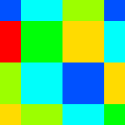
nearest-neighbor interpolation

for the nearest-neighbor interpolation,

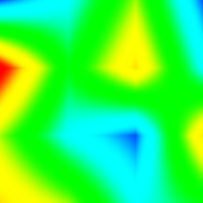
bilinear interpolation

for the bilinear interpolation, and:

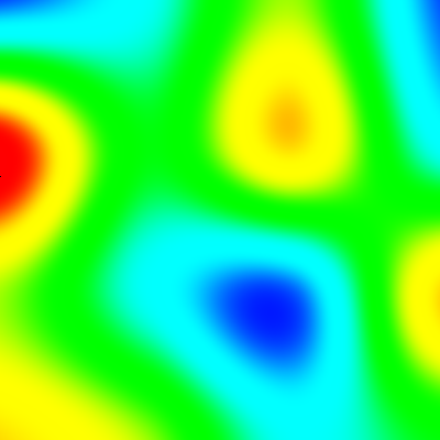
bicubic interpolation

for the bicubic interpolation. I know, the colors are toxic. Of course, with the draw() that I've given above the result should be solid black for each mouse click; to see the interpolations in action, comment the call to interp1().

In the next post I'll show a number of massages performed on interp0().

2012-01-06

Perlin's Simplex Noise

Graphics pioneer Ken Perlin is well-known for his work on procedural generation of textures. Recently he rewrote his classic Noise algorithm to reduce the complexity of generating pseudorandom gradients in higher dimensions by transforming a problem on N-cells to one on N-simplices. I couldn't find on his NYU home page a write-up by his own hand; apparently the only implementation exists in his Java applet. There is a well-known exegesis by Stefan Gustavson that completely rewrites the algorithm; I've also found a write-up by Perlin himself in a collection of course notes. The latter shows an extremely terse implementation in Java (Appendix B) that purports to correspond directly with hardware operations implemented in a specialized pipelined processor. I'll show an unraveled re-implementation of that Java algorithm that exactly corresponds to Prof. Perlin's, in the sense that the outputs are the same, but with the magic hopefully explained clearly. I will assume, however, that you are familiar with the original algorithm; if not, read Gustavson's analysis for a clear introduction to its workings.


The key to Perlin's Noise is that it interpolates pseudo-random gradients attached to lattice points. In the original algorithm, those gradients are computed by successive lookups using a permutation table. The new algorithm is geared towards an 8.8 fixed-point format; instead of tables it uses bit-slicing operations to compute two pseudo-random 3-bit hashes from the lattice points:


let patterns = [| 0o25; 0o70; 0o62; 0o54; 0o15; 0o23; 0o07; 0o52 |]

let btst n b = (n lsr b) land 1

let bmix i j k b = patterns.((btst i b lsl 2) lor (btst j b lsl 1) lor (btst k b))

let shuffle (i, j, k) =
  bmix i j k 0 + bmix j k i 1 + bmix k i j 2 + bmix i j k 3 +
  bmix j k i 4 + bmix k i j 5 + bmix i j k 6 + bmix j k i 7

I've expressed the patterns in octal to stress the fact that the result is a 6-bit number. btst simlpy extracts the b-th bit from n. bmix takes a 3-bit slice from the b-th bits of i, j and k, in that order, and uses it to index on patterns. shuffle adds up bmixes of eight circular rotations of (i, j, k) for each bit 0, 1 … 7. The procedure seems rather ad-hoc, but in fact produces rather well-distributed 3-bit fields among all the (28)3 = 16 Mi combinations of (i, j, k):


NP[Lower 3 bits = N]P[Upper 3 bits = N]
00.1244812011718750.125709712505340576
10.12536621093750.126831173896789551
20.1250.128595232963562
30.12463378906250.127514779567718506
40.1255187988281250.123155772686004639
50.12463378906250.120522260665893555
60.1250.12257838249206543
70.12536621093750.125092685222625732

These 3-bit hashes are used to compute a magnitude for vector (x, y, z) by selecting each coordinate with probability 3/4, applying a random sign to each with probability 1/2 and adding the resulting values:


let magnitude h (x, y, z) =
  let p, q, r = match h land 7 with
  | 0 -> z , x , y
  | 1 -> x , y , 0.
  | 2 -> y , z , 0.
  | 3 -> z , x , 0.
  | 4 -> z , x , y
  | 5 -> x , 0., z
  | 6 -> y , 0., x
  | 7 -> z , 0., y
  | _ -> assert false
  in match (h lsr 3) land 7 with
  | 0 -> -. p -. q +. r
  | 1 -> +. p -. q -. r
  | 2 -> -. p +. q -. r
  | 3 -> +. p +. q +. r
  | 4 -> +. p +. q -. r
  | 5 -> -. p +. q +. r
  | 6 -> +. p -. q +. r
  | 7 -> -. p -. q -. r
  | _ -> assert false

This amounts to finding the dot product of the vector (x, y, z) with a random gradient on the unit cell. Generating all combinations and extracting the gradient vectors we get the following diagram:


Distribution of the random basis vectors

Each dot shows the frequency with which that vector is selected; the diagonal vectors (±1, ±1, ±1) occur half as frequently as the mid-edge vectors (±1, ±1, 0) —and rotations—, to account for their greater magnitude and thus weight. All this is done without multiplying! If you study Perlin's paper and code, you will notice that he uses bit operations to select each of the x, y and z coordinates and to add or subtract them, to avoid using tables; however, the code doesn't quite correspond to the explanation given in the text. I've unrolled the conditionals into two jump tables in a way that duplicates the effect of the code; thus the first jump table is not equivalent to the one given in the text.


The key to the efficiency of this algorithm is not just in the use of bit operations for generating pseudo-random gradients but in the subdivision strategy used to combine them in ℝN. In the original algorithm, each of the 2N vertices in the N-cell are associated with a gradient which is cubically interpolated between pairs of hyperplanes. This not only generates visual artifacts since the interpolation scheme is not C²-continuous, it requires O(2N) work. The new algorithm mitigates the first problem by using a quartic interpolant, and solves the second by decomposing the N-cell into N! simplices:


let simplices = [|
[| (0,0,0); (1,0,0); (1,1,0); (1,1,1) |];
[| (0,0,0); (1,0,0); (1,0,1); (1,1,1) |];
[| (0,0,0); (0,1,0); (1,1,0); (1,1,1) |];
[| (0,0,0); (0,1,0); (0,1,1); (1,1,1) |];
[| (0,0,0); (0,0,1); (1,0,1); (1,1,1) |];
[| (0,0,0); (0,0,1); (0,1,1); (1,1,1) |]
|]

This requires interpolating among N + 1 vertices taken in pairs, for O(N²) work total. The simplex in which a point (u, v, w) in the unit cell lies is determined by the permutation index of coordinates (u, v, w):


let permindex (u, v, w) =
  if u >= w then
    if u >= v then
      if v >= w then 0 else 1
    else 2
  else
  if v >= w then 3 else
  if u >= v then 4 else 5

Perlin's code uses a different method to directly travel along the simplex edges by incrementing each coordinate according to the permutation index; I've opted for using a table to simplify the code and eliminate the need for global variables. Each point (x, y, z) is decomposed into a sum of a lattice vector (i, j, k) and a point in the unit cell (u, v, w). To account for the different volumes in the simplicial decomposition of the unit N-cell, the vectors are skewed:


let int x =
  if x < 0. then pred (truncate x) else truncate x

let skew (x, y, z) =
  let s = (x +. y +. z) /. 3. in
  let i = int (x +. s)
  and j = int (y +. s)
  and k = int (z +. s) in
  (i, j, k)

and unskewed:


let unskew (x, y, z) (i, j, k) =
  let s = float (i + j + k) /. 6. in
  let u = x -. float i +. s
  and v = y -. float j +. s
  and w = z -. float k +. s in
  (u, v, w)

along the main diagonal of the N-cell. This amounts to a change of basis between a cubic and a tetrahedral grid and back. In general, the skewing factor is (√(N+1) - 1)/N and the unskewing factor is (N + 1 - √(N+1))/(N(N+1)). A couple of simple functions will simplify the main routine:


let norm2 (x, y, z) = x *. x +. y *. y +. z *. z

let addi3 (i, j, k) (i', j', k') = (i + i', j + j', k + k')

Now given a point p, noise finds the lattice vector l and the unit-cell coordinates x corresponding to it. It then selects the simplex s corresponding to x. Then, for each of its vertices v it finds the simplicial coordinates y of x relative to v. It computes in t a radial basis for y such that only the gradients attached to the simplex's vertices contribute to the final result. If it does, it computes the hash h corresponding to v, uses it to find the pseudo-random gradient applied to y and accumulates the corresponding contribution for this vertex:


let noise p =
  let l = skew   p   in
  let x = unskew p l in
  let s = simplices.(permindex x) in
  let f = ref 0. in
  for i = 0 to 3 do
    let v = s.(i) in
    let y = unskew x v in
    let t = 0.6 -. norm2 y in
    if t > 0. then
      let h = shuffle (addi3 l v) in
      let t = t *. t in
      f := !f +. 8. *. t *. t *. magnitude h y
  done;
  !f

That's it. noise returns a floating-point number in the interval [-1, 1]; in order to use it in pixmaps it is frequently more useful to rescale it to an unsigned byte:


let clampb n =
  (n lor ((255-n) asr (Sys.word_size-2))) land lnot (n asr (Sys.word_size-2)) land 255

let rescale f =
  clampb (int (0.5 +. ldexp (f +. 1.) 7))

clampb is a nice little branchless routine to constrain an integer to the range [0, 255]. Note that in OCaml, integers are Sys.word_size - 1 bits long; in Java, for instance, the code would be:


public static int clampb(int n) {
  return (n | ((255-n) >>> 31)) & ~(n >>> 31) & 255;
}

(teasing that code apart is a nice exercise in bit twiddling.) This implementation produces the same result, pixel for pixel, as Perlin's code. This is a slice in the interval (-2, -2, 0)–(2, 2, 0) as a GIF file computed with this code:


Perlin simplex noise in the interval (-2, -2, 0)-(2, 2, 0) computed in OCaml

and this is the same slice as a PNG file computed in Java with the class given by Perlin in his Appendix B:


Perlin simplex noise in the interval (-2, -2, 0)-(2, 2, 0) computed in Java

There are two avenues open for further explorations of this algorithm. The first is to generalize it to an arbitrary number of dimensions; Gustavson's paper is a good starting point for that. The other is to go further with Perlin's original intention of building a hardware generator and eliminate the use of floating-point operations. This is mostly mechanical, except for the calculation of t in the inner loop, which requires at least a 0.24 fixed-point format.

2011-12-29

Vose's Alias Method

This is a note regarding the implementation of Vose's Method to construct the alias tables for non-uniform discrete probability sampling presented by Keith Schwartz (as of 2011-12-29). Mr. Schwartz otherwise very informative write-up contains an error in the presentation of the Method. Step 5 of the algorithm fails if the Small list is nonempty but the Large list is. This can happen either:


  1. if the initial probabilities sum to less than 1, or
  2. if updating in step 5.5 the Large probability results in cancellation so that pg results in an approximation less than its true value

The first case can be mitigated by scaling by n / ∑ pj in step 3. The second case can be mitigated by replacing 5.5 by "Set pg := (pg + pl) - 1." In any case, there is no proof that the algorithm as shown is correct, which is not the case for Vose's presentation. In the interest of correctness and completeness, here is an OCaml implementation of Vose's Method:


type alias = { n : int; prob : float array; alias : int array; }

let alias pa =
  let rec split pa n j (small, large as part) =
    if j == n then part else
    if pa.(j) > 1.
      then split pa n (succ j) (     small, j :: large)
      else split pa n (succ j) (j :: small,      large)
  in
  let rec init r pa part = match part with
  | j :: small, k :: large ->
    r.prob.(j)  <- pa.(j);
    r.alias.(j) <- k;
    pa.(k)      <- (pa.(k) +. pa.(j)) -. 1.;
    if pa.(k) > 1.
      then init r pa (small, k :: large)
      else init r pa (k :: small, large)
  | j :: small, []         ->
    r.prob.(j) <- 1.;
    init r pa (small, [])
  | []        , k :: large ->
    r.prob.(k) <- 1.;
    init r pa ([], large)
  | []        , []         -> r
  in
  let n  = Array.length pa in
  if n == 0 then invalid_arg "alias" else
  let sc = float n /. Array.fold_left (fun s p ->
    if p < 0. then invalid_arg "alias" else
    s +. p) 0. pa in
  let sa = Array.map (( *. ) sc) pa in
  let r  = { n; prob = Array.make n 0.; alias = Array.make n (-1); } in
  init r sa (split sa n 0 ([], []))

let choose r =
  let p, e = modf (Random.float (float r.n)) in
  let j = truncate e in
  if p <= r.prob.(j) then j else r.alias.(j)

Since this algorithm is recursive, it might not be immediately obvious how to translate it to more mainstream languages. A perhaps more faithful rendition in rather low-level Java is the following:


import java.util.Random;

public class Vose {
  private final Random random;
  private final int limit;
  private final double[] prob;
  private final int[] alias;

  public Vose(final double[] pa) {
    this(pa, new Random());
  }

  public int getLimit() {
    return limit;
  }

  public Vose(final double[] pa, final Random random) {
    final int limit = pa.length;
    if (limit == 0)
      throw new IllegalArgumentException("Vose");
    double sum = 0;
    for (int j = 0; j != limit; j++) {
      if (pa[j] < 0)
        throw new IllegalArgumentException("Vose");
      sum += pa[j];
    }
    final double scale = (double) limit / sum;
    final double[] sa = new double[limit];
    for (int j = 0; j != limit; j++)
      sa[j] = pa[j] * scale;

    this.random = random;
    this.limit  = limit;
    this.prob   = new double[limit];
    this.alias  = new int[limit];
    init(sa);
  }

  private void init(final double[] sa) {
    final int[] small = new int[limit];
    final int[] large = new int[limit];
    int ns = 0;
    int nl = 0;
    for (int j = 0; j != limit; j++)
      if (sa[j] > 1)
        large[nl++] = j;
      else
        small[ns++] = j;
    while (ns != 0 && nl != 0) {
      final int j = small[--ns];
      final int k = large[--nl];
      prob[j]  = sa[j];
      alias[j] = k;
      sa[k]    = (sa[k] + sa[j]) - 1; // sic
      if (sa[k] > 1)
        large[nl++] = k;
      else
        small[ns++] = k;
    }
    while (ns != 0)
      prob[small[--ns]] = 1;
    while (nl != 0)
      prob[large[--nl]] = 1;
  }

  public int choose() {
    final double u = limit * random.nextDouble();
    final int    j = (int) Math.floor(u);
    final double p = u - (double) j;
    return p <= prob[j] ? j : alias[j];
  }
}

In all generality, it is sufficient that the "probabilities" be non-negative, since dividing the values by the mean normalizes them so that the conditions of the Method are satisfied.


References


  1. Michael D. Vose. A Linear Algorithm For Generating Random Numbers With a Given Distribution, IEEE TRANSACTIONS ON SOFTWARE ENGINEERING VOL. 17, NO. 9 SEPTEMBER 1991. Online.